T01: Single Cell Analysis

Hint

By the end of this notebook, you will be able to:

• Load neuronal reconstructions from multiple sources (local files and demo datasets)

• Visualize neuronal morphology using PySNT’s display function

• Extract basic quantitative measurements from neuronal trees using TreeStatistics and its variants

• Visualize quantitative measurements using color mappers

• Generate histograms of morphological features

• Apply statistical fitting to morphological distributions

• Transform neuronal reconstructions using geometric operations and modifications

• Work with SWC-type labels to identify and isolate different cellular compartments

• Work with subsets of reconstruction nodes (point clouds)

Estimated Time: 20-30 minutes

Note

Make sure to read these resources before running this notebook:

• Install - Installation instructions

• Quickstart - Get started quickly

• Overview - Tour of pysnt’s architecture

Setup and Initialization

As always, we start by initializing pysnt. We’ll also set some generic options suitable for notebook execution:

import pysnt
pysnt.set_option('java.logging.level', 'Error') # Set logging level to 'Error' to reduce console output (see Overview for details)
pysnt.set_option('display.chart_format', 'svg') # SVG plots and histograms
pysnt.set_option('display.chart_dpi', 150) # Rendering resolution

import pysnt
pysnt.initialize()

Loading a Tree

As mentioned in the Quickstart guide, in SNT a neuronal reconstruction is a pysnt.Tree object.

There are multiple ways to load a tree:

• From a local file

• From a remote database: Using loaders for major online databases: FlyCircuit, InsectBrain, NeuroMorpho, MouseLight

• From a demo dataset

To load a local file we can use:

## Loading from local file
from pysnt import Tree
try:
    tree = Tree('/path/to/a/swc/file.swc')
    tree = Tree('/path/to/a/swc/file.swc', "axon") # will only load axon-tagged nodes
except FileNotFoundError as e: # Handle Python-exceptions first
    print(f"File does not exist: {e}")
except Exception as e:  # Catch SNT exceptions
    print(f"Unexpected error: {e}")

Unexpected error: java.lang.IllegalArgumentException: File is not available: /path/to/a/swc/file.swc

(which of course will fail, since these files don’t exist).

We will access reconstruction files from remote databases in subsequent tutorials. For now, let’s use some demo datasets. We’ll use pysnt.SNTService: SNT’s SciJava service that provides convenience access to common operations as well as the running SNT instance:

from pysnt import SNTService
snt_service = SNTService()
tree = snt_service.demoTree('pyramidal')  # or 'OP1' (DIADEM dataset), or 'DG' (Dentate gyrus granule cell), or 'fractal' for an L-system toy neuron
print(f"Demo tree loaded: {tree.getLabel()}")

Demo tree loaded: AA0001

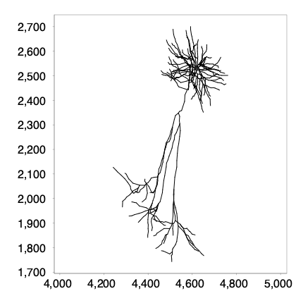
Let’s display it! We could use one of SNT’s advanced viewers like Reconstruction Viewer (pysnt.viewer.Viewer3D) or Reconstruction Plotter (pysnt.viewer.Viewer2D), but for now let’s simply show the Tree’s skeleton. We can use display(): it is a convenient function that allows us to automagically display all sorts of objects: from text, to tables, to – as we’ll see in subsequent tutorials – 3D scenes:

pysnt.display(tree)

[SNTUtils] Retrieving org.scijava.Context...

[INFO] [SNT] 116 scijava services loaded

{'type': matplotlib.figure.Figure,
 'data': <Figure size 400x400 with 1 Axes>,
 'metadata': {'source_type': 'SNTChart',
  'format': 'svg',
  'scale': 1.0,
  'is_combined': False,
  'title': 'AA0001',
  'containsValidData': True,
  'isLegendVisible': True},
 'error': None}

Measuring a Tree

Most simply, a Tree can be measured using pysnt.analysis.TreeStatistics. Further specialized measurements (Strahler, Sholl, graph analysis, persistence homology, etc.) are retrieved using other classes in pysnt.analysis. We will discuss those in subsequent tutorials. Here we’ll focus on TreeStatistics. We construct an instance like so:

from pysnt.analysis import TreeStatistics
t_stats = TreeStatistics(tree)

TreeStatistics provides a variety of single value measurements as well as distribution statistics. Single value metrics:

cable = t_stats.getCableLength()
print("The cable length is %d micrometers" % cable)
n_bps = len(t_stats.getBranchPoints())
print(f"The no. of branch points is: {n_bps}")

The cable length is 13718 micrometers
The no. of branch points is: 82

Tip

You can use Python’s help function to know more about a class or method, e.g.,: help(TreeStatistics)

To see the full list of supported metrics, we can use getMetrics(choice), where ‘choice’ is either ‘safe’ (metrics that do not require the Tree to validate as an acyclic rooted graph), ‘common’ (most frequently used), ‘quick’ (used by SNT’s Quick Measure… command), or ‘all’:

print("The following metrics are available:")
metrics = t_stats.getMetrics('all')
for i in range(0, len(metrics), 2):
    left = f"{i+1:3d}. {metrics[i]}" if i < len(metrics) else ""
    right = f"{i+2:3d}. {metrics[i+1]}" if i+1 < len(metrics) else ""
    print(f'{left:<60}{right}')

The following metrics are available:
  1. Longest shortest path: Extension angle                   2. Longest shortest path: Extension angle XY
  3. Longest shortest path: Extension angle XZ                4. Longest shortest path: Extension angle ZY
  5. Branch contraction                                       6. Branch fractal dimension
  7. Branch length                                            8. Branch mean radius
  9. Branch surface area                                     10. Branch volume
 11. Complexity index: ACI                                   12. Complexity index: DCI
 13. Convex hull: Boundary size                              14. Convex hull: Boxivity
 15. Convex hull: Centroid-root distance                     16. Convex hull: Elongation
 17. Convex hull: Roundness                                  18. Convex hull: Size
 19. Convex hull: Compactness                                20. Convex hull: Eccentricity
 21. Depth                                                   22. Branch extension angle
 23. Branch extension angle (Rel.)                           24. Branch extension angle XY
 25. Branch extension angle XZ                               26. Branch extension angle ZY
 27. Inner branches: Extension angle                         28. Inner branches: Extension angle (Rel.)
 29. Inner branches: Extension angle XY                      30. Inner branches: Extension angle XZ
 31. Inner branches: Extension angle ZY                      32. Primary branches: Extension angle
 33. Primary branches: Extension angle XY                    34. Primary branches: Extension angle XZ
 35. Primary branches: Extension angle ZY                    36. Terminal branches: Extension angle
 37. Terminal branches: Extension angle (Rel.)               38. Terminal branches: Extension angle XY
 39. Terminal branches: Extension angle XZ                   40. Terminal branches: Extension angle ZY
 41. Longest shortest path: Length                           42. Height
 43. Inner branches: Length                                  44. Internode angle
 45. Internode distance                                      46. Internode distance (squared)
 47. Cable length                                            48. No. of branch nodes (branch fragmentation)
 49. No. of branch points                                    50. No. of branches
 51. No. of fitted paths                                     52. No. of inner branches
 53. No. of nodes                                            54. No. of path nodes (path fragmentation)
 55. No. of paths                                            56. No. of primary branches
 57. No. of spines/varicosities                              58. No. of terminal branches
 59. No. of tips                                             60. Node radius
 61. Partition asymmetry                                     62. Path channel
 63. Path contraction                                        64. Path fractal dimension
 65. Path frame                                              66. Path extension angle
 67. Path extension angle (Rel.)                             68. Path extension angle XY
 69. Path extension angle XZ                                 70. Path extension angle ZY
 71. Path length                                             72. Path mean radius
 73. Path spine/varicosity density                           74. No. of spines/varicosities per path
 75. Path order                                              76. Path surface area
 77. Path volume                                             78. Primary branches: Length
 79. Remote bif. angles                                      80. Root angles: Balancing factor
 81. Root angles: Centripetal bias                           82. Root angles: Mean direction
 83. Sholl: Decay                                            84. Sholl: Kurtosis
 85. Sholl: Max (fitted)                                     86. Sholl: Max (fitted) radius
 87. Sholl: Max                                              88. Sholl: Mean
 89. Sholl: No. maxima                                       90. Sholl: No. secondary maxima
 91. Sholl: Degree of Polynomial fit                         92. Sholl: Ramification index
 93. Sholl: Skeweness                                        94. Sholl: Sum
 95. Horton-Strahler root number                             96. Horton-Strahler bifurcation ratio
 97. Surface area                                            98. Terminal branches: Length
 99. Node intensity values                                  100. Volume
101. Width                                                  102. X coordinates
103. Y coordinates                                          104. Z coordinates

These metrics can be used to retrieve computations, distributions, etc.

metric = "Internode distance" #fuzzy matching is supported so we can abbreviate distance
summary_stats = t_stats.getSummaryStats(metric)
print("The average inter-node distance is %d µm" % summary_stats.getMean())
print("The standard deviation is %d µm" % summary_stats.getStandardDeviation())

The average inter-node distance is 14 µm
The standard deviation is 6 µm

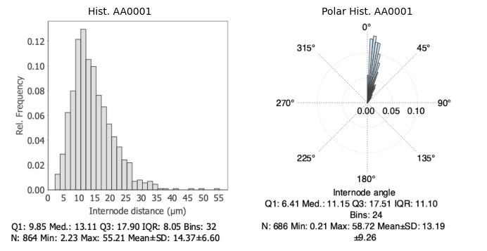
A neat feature of SNT, is that it is quick and convenient to inspect quantitative data. E.g., one can plot histograms directly:

Note

The following cell may produce verbose logging output from the underlying libraries during histogram generation. This output can be safely ignored.

hist1 = t_stats.getHistogram('internode distance')
hist2 = t_stats.getPolarHistogram('internode angle')
pysnt.display([hist1, hist2])

[main] INFO smile.stat.distribution.GaussianMixture - The BIC of Mixture(1)[1.00 x Gaussian Distribution(14.3722, 6.6011)] = -2862.7968
[main] INFO smile.stat.distribution.GaussianMixture - The BIC of Mixture(2)[0.69 x Gaussian Distribution(13.5866, 5.9980) + 0.31 x Gaussian Distribution(16.1047, 7.4705)] = -2851.4582

{'type': matplotlib.figure.Figure,
 'data': <Figure size 700x350 with 2 Axes>,
 'metadata': {'source_type': 'SNTChart_List',
  'sntchart_count': 2,
  'displayed_count': 2,
  'panel_layout': 'auto',
  'title': None},
 'error': None}

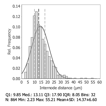
Did you notice GaussianMixture debug message in the background? It reflects background computations on the distribution. While SNT is not a statistical package, it does offer entry points for detailed data inspection. E.g., one can fit the histogram distribution to a Gaussian/ Gaussian mixture model directly:

hist1.setGaussianFitVisible(True) # or hist1.setGMMFitVisible(True) for Gaussian mixture model
hist1.setQuartilesVisible(True) # Display 1st quartile, Median, and 3rd quartile
pysnt.display(hist1)

{'type': matplotlib.figure.Figure,
 'data': <Figure size 400x400 with 1 Axes>,
 'metadata': {'source_type': 'SNTChart',
  'format': 'svg',
  'scale': 1.0,
  'is_combined': False,
  'title': 'Hist. AA0001',
  'containsValidData': True,
  'isLegendVisible': False},
 'error': None}

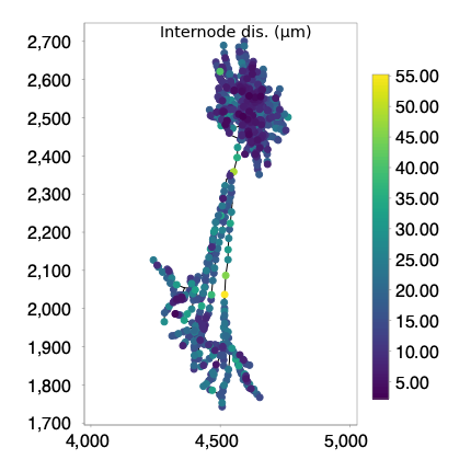
We can actually ‘overlay’ the distribution on the reconstruction itself, by means of a ColorMapper. Color mappers map quantitative traits to reconstructions. Because we are handling Trees, we can use TreeColorMapper.

To visualize the nodes we need to use a viewer. We can use Reconstruction Plotter (i.e., pysnt.viewer.Viewer2D). We will use 3D viewers in subsequent tutorials, but for now we’ll use the 2D viewer because it is quite simple:

from pysnt.analysis import TreeColorMapper
from pysnt.viewer import Viewer2D

# assign colors
color_mapper = TreeColorMapper()
color_mapper.map(tree, 'internode distance', 'viridis') # tree, metric, LUT/colormap (NB: some LUTs are case-sensitive)

# assemble viewer
viewer = Viewer2D()
viewer.add(tree)
viewer.addColorBarLegend(color_mapper)

# remove mapping: restore original colors
color_mapper.unMap(tree)

pysnt.display(viewer, title='Internode Dist. (µm)')

{'type': matplotlib.figure.Figure,
 'data': <Figure size 400x400 with 1 Axes>,
 'metadata': {'source_type': 'SNTChart',
  'format': 'svg',
  'scale': 1.0,
  'is_combined': False,
  'title': 'Reconstruction Plotter',
  'containsValidData': True,
  'isLegendVisible': True},
 'error': None}

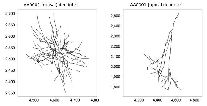
Cellular Compartments

If the reconstruction nodes are tagged with SWC-type flags, it is possible to retrieve the cellular compartments (axon, basal dendrites, etc).

# Find out how many compartments exist
types = tree.getSWCTypeNames(True) # include soma?
print(f"Found {len(types)} SWC type labels: {types}")

# Retrieve each compartment (as subtree)
all_sub_trees = []
for type in types:
    sub_tree = tree.subTree(type)
    if (len(sub_tree.getNodes()) == 1):
        print(f"{type} has only a single node. Skipping visualization")
        continue
    all_sub_trees.append(sub_tree)

# Display subtrees
pysnt.display(all_sub_trees)

Found 3 SWC type labels: [(basal) dendrite, apical dendrite, soma]
soma has only a single node. Skipping visualization

{'type': matplotlib.figure.Figure,
 'data': <Figure size 700x350 with 2 Axes>,
 'metadata': {'source_type': 'SNTChart_List',
  'sntchart_count': 2,
  'displayed_count': 2,
  'panel_layout': 'auto',
  'title': None},
 'error': None}

Subsets of Nodes

Subsets of nodes can be studied using NodeStatistics, a TreeStatistics variant that operates on collections of nodes, i.e., point clouds.

from pysnt.analysis import NodeStatistics

node_subsets = [tree.getBPs(), tree.getTips()] # list of branch points (BPs) and end points (tips)
histograms = []
for subset in node_subsets:
    node_stats = NodeStatistics(subset)
    hist = node_stats.getHistogram('nearest neighbor distance')
    hist.setGaussianFitVisible(True)
    histograms.append(hist)
    
# pysnt.set_option('display.chart_format', 'pdf')

pysnt.set_option('display.chart_format', 'svg')
pysnt.display(histograms, panel_titles=['Branch Points', 'Tips'])

[main] INFO smile.stat.distribution.GaussianMixture - The BIC of Mixture(1)[1.00 x Gaussian Distribution(23.6177, 20.2284)] = -366.8408
[main] INFO smile.stat.distribution.GaussianMixture - The BIC of Mixture(2)[0.69 x Gaussian Distribution(19.2077, 15.0684) + 0.31 x Gaussian Distribution(33.3124, 25.6294)] = -362.6232

{'type': matplotlib.figure.Figure,
 'data': <Figure size 700x350 with 2 Axes>,
 'metadata': {'source_type': 'SNTChart_List',
  'sntchart_count': 2,
  'displayed_count': 2,
  'panel_layout': 'auto',
  'title': None},
 'error': None}

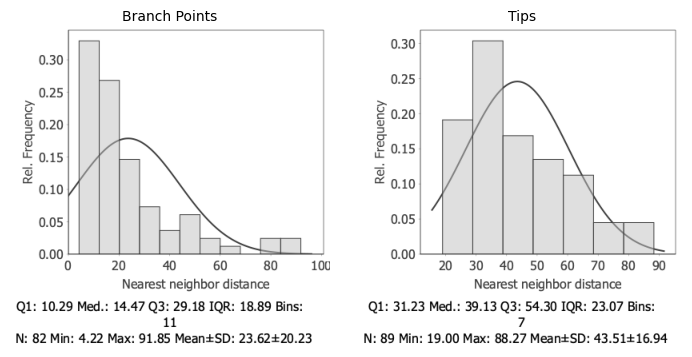
The distribution of nearest-neighbor distances for branch points is strongly right-skewed, indicating that many branch points are tightly packed together within 30µm. The long tail extending toward larger distances (up to about 90µm) shows a few isolated points that are much farther apart.

The tips have a broader and more symmetric distribution compared to the branch points: Tips are spaced farther apart on average and more evenly distributed in space than branch points.

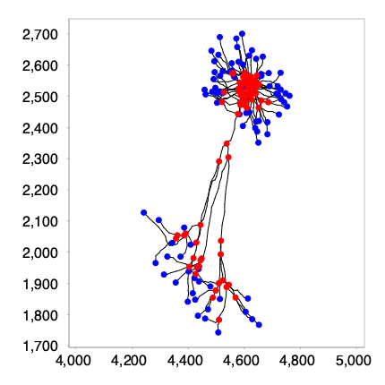
We can visualize the nodes by assembling a simple 2D scene:

viewer = Viewer2D()
viewer.add(tree)
viewer.addNodes(tree.getBPs(), 'red', 'branch points')
viewer.addNodes(tree.getTips(), 'blue', 'tips')
pysnt.display(viewer)

{'type': matplotlib.figure.Figure,
 'data': <Figure size 400x400 with 1 Axes>,
 'metadata': {'source_type': 'SNTChart',
  'format': 'svg',
  'scale': 1.0,
  'is_combined': False,
  'title': 'Reconstruction Plotter',
  'containsValidData': True,
  'isLegendVisible': True},
 'error': None}

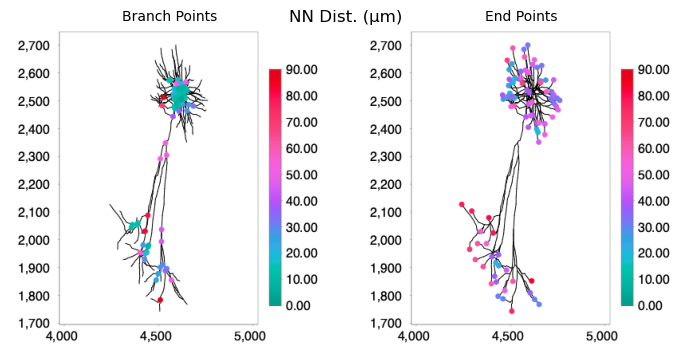
Which illustrates our previous assessment. To find out which branch points are much farther apart, we can map the distances into the structure. Because we used NodeStatistics, we now use NodeColorMapper as color mapper:

from pysnt.analysis import NodeColorMapper

node_subsets = [tree.getBPs(), tree.getTips()]
viewers = []
for subset in node_subsets:
    node_stats = NodeStatistics(subset)
    node_mapper = NodeColorMapper(node_stats)
    node_mapper.setMinMax(0, 90) # set the same boundaries for both mappers (in µm)
    node_mapper.map("nearest neighbor distance", "ice") # mapping metric, lut/colormap LUT/colormap (NB: some LUTs are case-sensitive)
    
    # Assemble a 2D scene as before
    viewer = Viewer2D()
    viewer.add(tree)
    viewer.addNodes(node_mapper.getNodesByColor())
    viewer.addColorBarLegend(node_mapper)
    viewers.append(viewer)

pysnt.display(viewers, title="NN Dist. (µm)", panel_titles=["Branch Points", "End Points"])

{'type': matplotlib.figure.Figure,
 'data': <Figure size 700x350 with 2 Axes>,
 'metadata': {'source_type': 'Viewer2D_List',
  'viewer2d_count': 2,
  'displayed_count': 2,
  'panel_layout': 'auto',
  'title': 'NN Dist. (µm)'},
 'error': None}

Transforming Trees

You should be able to use auto-completion on your IDE to explore some of the transformation options available. Transformations occur in place, so we’ll work on a copy of the initial tree. Here are some examples.

tree_transformed = tree.clone() # Duplicate Tree
tree_transformed.rotate(Tree.Z_AXIS, 90) # Rotate around Z axis by 90 degrees
tree_transformed.translate(100, 100, 100) # Translate by 100, 100, 100 µm in X,Y,Z
tree_transformed.scale(1.5, 1.5, 3.0) # Scale by 1.50 in XY; 3.0 in Z
pysnt.display(tree_transformed)

{'type': matplotlib.figure.Figure,
 'data': <Figure size 400x400 with 1 Axes>,
 'metadata': {'source_type': 'SNTChart',
  'format': 'svg',
  'scale': 1.0,
  'is_combined': False,
  'title': 'AA0001',
  'containsValidData': True,
  'isLegendVisible': True},
 'error': None}

There are also transform() and transformedCopy() methods that allow for standardized transformations using space-separated flags:

Projection flags:

• zy: ZY projection

• xz: XZ projection

Translation flags:

• zero-origin: Tree is translated so that its root has (0,0,0) coordinates

Rotation flags:

• upright-geodesic: Tree is rotated to vertically align its “longest shortest path” (in graph theory this is called the longest geodesic, or graph diameter). Sometimes it is also called the neuron’s backbone or spine

• upright-tips: Tree is rotated to vertically align its [root, tips centroid] vector

• r#: With # specifying a positive integer (e.g., r90): Tree is rotated by the specified angle (in degrees)

Example:

tree_transformed = tree
tree_transformed = tree.transformedCopy("upright-geodesic") # Project into xz plane + rotate vertically until the longest path in the tree graph is vertical
pysnt.display(tree_transformed)

{'type': matplotlib.figure.Figure,
 'data': <Figure size 400x400 with 1 Axes>,
 'metadata': {'source_type': 'SNTChart',
  'format': 'svg',
  'scale': 1.0,
  'is_combined': False,
  'title': 'AA0001',
  'containsValidData': True,
  'isLegendVisible': True},
 'error': None}

Measuring a Group of Trees

Multiple trees are analyzed using pysnt.analysis.MultiTreeStatistics, a TreeStatistics variant that analyses trees belonging to a common group. Its usage is rather similar to TreeStatistics.

We start by importing a group of Trees. As usual we could use local files, e.g., using:

• Tree.listFromDir('/path/to/a/directory/') to load all reconstruction files in the directory

• Tree.listFromDir('/path/to/a/directory/', 'pattern') to load all reconstruction files in the directory with pattern in their filename

• Tree.listFromDir('/path/to/a/directory/', 'pattern', 'swc_type_label') to load all reconstruction files in the directory with pattern in their filename, with swc_type_label identifying the compartments to be imported ‘soma’, ‘axon’, ‘dendrite’, ‘all’, etc.

As before, we’ll use a small demo dataset for now, from which we can instantiate a MultiTreeStatistics instance:

from pysnt.analysis import MultiTreeStatistics
trees = snt_service.demoTrees() # dendrites from 4 pyramidal cells from the MouseLight database
m_stats = MultiTreeStatistics(trees)
m_stats.setLabel("multiple trees analysis") # Optional: we can set a unifying label to be used in reports, etc.

Subsequent analysis works the same as with TreeStatistics:

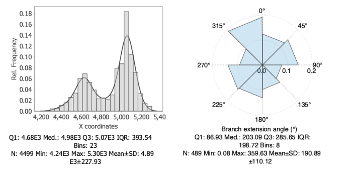
hist1 = m_stats.getHistogram("x coordinates")
hist1.setGMMFitVisible(True)
hist2 = m_stats.getPolarHistogram("branch extension angle")
pysnt.display([hist1, hist2], show_panel_titles=False)

[main] INFO smile.stat.distribution.GaussianMixture - The BIC of Mixture(1)[1.00 x Gaussian Distribution(4893.6491, 227.9298)] = -30816.9576
[main] INFO smile.stat.distribution.GaussianMixture - The BIC of Mixture(2)[0.42 x Gaussian Distribution(4811.8170, 236.9718) + 0.58 x Gaussian Distribution(4952.9253, 201.3027)] = -30775.8996

{'type': matplotlib.figure.Figure,
 'data': <Figure size 700x350 with 2 Axes>,
 'metadata': {'source_type': 'SNTChart_List',
  'sntchart_count': 2,
  'displayed_count': 2,
  'panel_layout': 'auto',
  'title': None},
 'error': None}

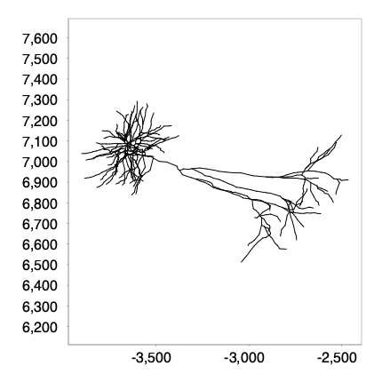
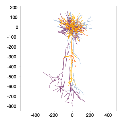
To display the group, we can use Reconstruction Plotter (i.e., Viewer2D) (we will use 3D viewers in the subsequent tutorials, but for now we’ll use the 2D viewer because it is quite simple):

from pysnt.viewer import Viewer2D
viewer = Viewer2D()
viewer.add(trees)
pysnt.display(viewer)

{'type': matplotlib.figure.Figure,
 'data': <Figure size 400x400 with 1 Axes>,
 'metadata': {'source_type': 'SNTChart',
  'format': 'svg',
  'scale': 1.0,
  'is_combined': False,
  'title': 'Reconstruction Plotter',
  'containsValidData': True,
  'isLegendVisible': True},
 'error': None}

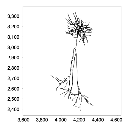
Using what we learned so far, we can display the cells in a more concise way:

trees_transformed = Tree.transform(trees, "zero-origin upright-geodesic", False) # Move all roots to (0,0,0) coordinate, rotate the cells so their main axis is vertical
viewer = Viewer2D()
viewer.add(trees_transformed)
pysnt.display(viewer)

{'type': matplotlib.figure.Figure,
 'data': <Figure size 400x400 with 1 Axes>,
 'metadata': {'source_type': 'SNTChart',
  'format': 'svg',
  'scale': 1.0,
  'is_combined': False,
  'title': 'Reconstruction Plotter',
  'containsValidData': True,
  'isLegendVisible': True},
 'error': None}

Measuring Groups of Trees

Instead of MultipleTreeStatistics, we now use GroupedTreeStatistics: The approach is similar to what we’ve been doing so far, with a minor difference: We will first initialize the class, then we’ll add our cell groups.

To define the cell groups, we’ll just split the cells we’ve been studying evenly into two sub-groups:

from pysnt.analysis import GroupedTreeStatistics
g_stats = GroupedTreeStatistics()

trees = snt_service.demoTrees() # retrieve demo trees
mid = len(trees) // 2 # group mid point
g_stats.addGroup(trees[:mid], "group 1") # assign first half to group 1
g_stats.addGroup(trees[mid:], "group 2") # assign second half to group 2

def get_histogram(metric):
    hist = g_stats.getHistogram(metric)
    hist.setGaussianFitVisible(True) 
    hist.setQuartilesVisible(True)
    return hist

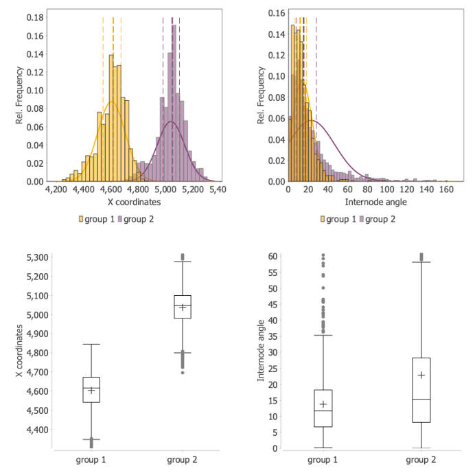
hist1 = get_histogram("x coordinates")
hist2 = get_histogram("internode angle")

[main] INFO smile.stat.distribution.GaussianMixture - The BIC of Mixture(1)[1.00 x Gaussian Distribution(4602.7220, 101.9468)] = -8981.2370
[main] INFO smile.stat.distribution.GaussianMixture - The BIC of Mixture(2)[0.43 x Gaussian Distribution(4574.4973, 107.9735) + 0.57 x Gaussian Distribution(4623.9380, 91.5477)] = -8972.1973
[main] INFO smile.stat.distribution.GaussianMixture - The BIC of Mixture(3)[0.21 x Gaussian Distribution(4527.5178, 110.7982) + 0.39 x Gaussian Distribution(4597.4964, 93.5217) + 0.40 x Gaussian Distribution(4646.1892, 78.7857)] = -8956.2239

Because we are working with group statistics, there are new functions to compare groups, including T-testing and ANOVA-testing. There are also some new plotting options:

plot1 = g_stats.getBoxPlot("x coordinates")
plot2 = g_stats.getBoxPlot("internode angle")
pysnt.display([hist1, hist2, plot1, plot2], show_panel_titles=False)

{'type': matplotlib.figure.Figure,
 'data': <Figure size 700x700 with 4 Axes>,
 'metadata': {'source_type': 'SNTChart_List',
  'sntchart_count': 4,
  'displayed_count': 4,
  'panel_layout': 'auto',
  'title': None},
 'error': None}

Internally, each group is assigned a MultiTreeStatistics instance, so we can use the same methods as before, and study each individual group:

for group in g_stats.getGroups():
    m_stats = g_stats.getGroupStats(group) # Retrieve the MultiTreeStatistics instance assigned to group
    print(f'Total no. of branch points in {group}: {len(m_stats.getBranches())}')

Total no. of branch points in group 1: 258
Total no. of branch points in group 2: 231

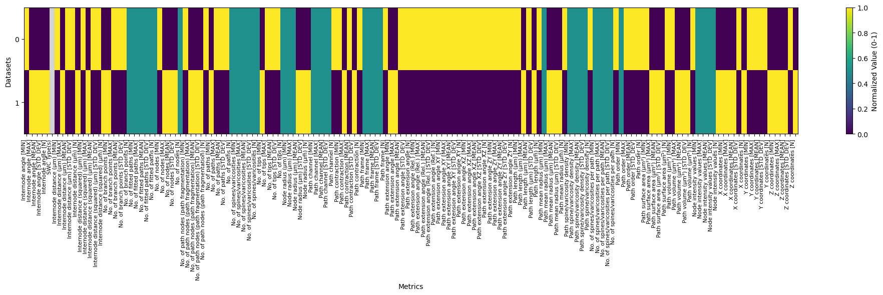
Actually, we can retrieve metrics in bulk like one would do from SNT’s Measurements prompt. We can exploit the fact that (Multi)TreeStatistics keeps an internal table of measurements. Thus, the strategy is as follows:

1. Define a master table to hold the data

2. Define a list of metrics

3. For each group, dump measurements into the master table

Let’s implement it:

from pysnt.analysis import SNTTable
master_table = SNTTable()

for group in g_stats.getGroups():
    m_stats = g_stats.getGroupStats(group)
    m_stats.setTable(master_table)
    metrics = m_stats.getMetrics('safe')
    m_stats.measure(group, metrics, False) # group description, list of metrics, whether measurements should consider SWC compartment (axon/dendrites)

pysnt.set_option('display.table_mode', 'heatmap_norm')
pysnt.display(master_table, figsize=(20, 6), title=None)

Column 'SWC Type(s)' is all NaN, skipping normalization
Column 'No. of branch points [N]' has no variation (min=max=2), setting to 0.5
Column 'No. of fitted paths [MIN]' has no variation (min=max=0.0), setting to 0.5
Column 'No. of fitted paths [MAX]' has no variation (min=max=0.0), setting to 0.5
Column 'No. of fitted paths [MEAN]' has no variation (min=max=0.0), setting to 0.5
Column 'No. of fitted paths [STD_DEV]' has no variation (min=max=0.0), setting to 0.5
Column 'No. of fitted paths [N]' has no variation (min=max=2), setting to 0.5
Column 'No. of nodes [N]' has no variation (min=max=2), setting to 0.5
Column 'No. of paths [N]' has no variation (min=max=2), setting to 0.5
Column 'No. of spines/varicosities [MIN]' has no variation (min=max=0.0), setting to 0.5
Column 'No. of spines/varicosities [MAX]' has no variation (min=max=0.0), setting to 0.5
Column 'No. of spines/varicosities [MEAN]' has no variation (min=max=0.0), setting to 0.5
Column 'No. of spines/varicosities [STD_DEV]' has no variation (min=max=0.0), setting to 0.5
Column 'No. of spines/varicosities [N]' has no variation (min=max=2), setting to 0.5
Column 'No. of tips [N]' has no variation (min=max=2), setting to 0.5
Column 'Node radius (µm) [MIN]' has no variation (min=max=0.5), setting to 0.5
Column 'Node radius (µm) [MAX]' has no variation (min=max=1.0), setting to 0.5
Column 'Path channel [MIN]' has no variation (min=max=1.0), setting to 0.5
Column 'Path channel [MAX]' has no variation (min=max=1.0), setting to 0.5
Column 'Path channel [MEAN]' has no variation (min=max=1.0), setting to 0.5
Column 'Path channel [STD_DEV]' has no variation (min=max=0.0), setting to 0.5
Column 'Path frame [MIN]' has no variation (min=max=1.0), setting to 0.5
Column 'Path frame [MAX]' has no variation (min=max=1.0), setting to 0.5
Column 'Path frame [MEAN]' has no variation (min=max=1.0), setting to 0.5
Column 'No. of branch points [N]' has no variation (min=max=2), setting to 0.5
Column 'No. of fitted paths [MIN]' has no variation (min=max=0.0), setting to 0.5
Column 'No. of fitted paths [MAX]' has no variation (min=max=0.0), setting to 0.5
Column 'No. of fitted paths [MEAN]' has no variation (min=max=0.0), setting to 0.5
Column 'No. of fitted paths [STD_DEV]' has no variation (min=max=0.0), setting to 0.5
Column 'No. of fitted paths [N]' has no variation (min=max=2), setting to 0.5
Column 'No. of nodes [N]' has no variation (min=max=2), setting to 0.5
Column 'No. of paths [N]' has no variation (min=max=2), setting to 0.5
Column 'No. of spines/varicosities [MIN]' has no variation (min=max=0.0), setting to 0.5
Column 'No. of spines/varicosities [MAX]' has no variation (min=max=0.0), setting to 0.5
Column 'No. of spines/varicosities [MEAN]' has no variation (min=max=0.0), setting to 0.5
Column 'No. of spines/varicosities [STD_DEV]' has no variation (min=max=0.0), setting to 0.5
Column 'No. of spines/varicosities [N]' has no variation (min=max=2), setting to 0.5
Column 'No. of tips [N]' has no variation (min=max=2), setting to 0.5
Column 'Node radius (µm) [MIN]' has no variation (min=max=0.5), setting to 0.5
Column 'Node radius (µm) [MAX]' has no variation (min=max=1.0), setting to 0.5
Column 'Path channel [MIN]' has no variation (min=max=1.0), setting to 0.5
Column 'Path channel [MAX]' has no variation (min=max=1.0), setting to 0.5
Column 'Path channel [MEAN]' has no variation (min=max=1.0), setting to 0.5
Column 'Path channel [STD_DEV]' has no variation (min=max=0.0), setting to 0.5
Column 'Path frame [MIN]' has no variation (min=max=1.0), setting to 0.5
Column 'Path frame [MAX]' has no variation (min=max=1.0), setting to 0.5
Column 'Path frame [MEAN]' has no variation (min=max=1.0), setting to 0.5
Column 'Path frame [STD_DEV]' has no variation (min=max=0.0), setting to 0.5
Column 'Path mean radius (µm) [MIN]' has no variation (min=max=0.5), setting to 0.5
Column 'Path spine/varicosity density [MIN]' has no variation (min=max=0.0), setting to 0.5
Column 'Path spine/varicosity density [MAX]' has no variation (min=max=0.0), setting to 0.5
Column 'Path spine/varicosity density [MEAN]' has no variation (min=max=0.0), setting to 0.5
Column 'Path spine/varicosity density [STD_DEV]' has no variation (min=max=0.0), setting to 0.5
Column 'No. of spines/varicosities per path [MIN]' has no variation (min=max=0.0), setting to 0.5
Column 'No. of spines/varicosities per path [MAX]' has no variation (min=max=0.0), setting to 0.5
Column 'No. of spines/varicosities per path [MEAN]' has no variation (min=max=0.0), setting to 0.5
Column 'No. of spines/varicosities per path [STD_DEV]' has no variation (min=max=0.0), setting to 0.5
Column 'Path order [MIN]' has no variation (min=max=1.0), setting to 0.5
Column 'Node intensity values [MIN]' has no variation (min=max=0.0), setting to 0.5
Column 'Node intensity values [MAX]' has no variation (min=max=0.0), setting to 0.5
Column 'Node intensity values [MEAN]' has no variation (min=max=0.0), setting to 0.5
Column 'Path frame [STD_DEV]' has no variation (min=max=0.0), setting to 0.5
Column 'Path mean radius (µm) [MIN]' has no variation (min=max=0.5), setting to 0.5
Column 'Path spine/varicosity density [MIN]' has no variation (min=max=0.0), setting to 0.5
Column 'Path spine/varicosity density [MAX]' has no variation (min=max=0.0), setting to 0.5
Column 'Path spine/varicosity density [MEAN]' has no variation (min=max=0.0), setting to 0.5
Column 'Path spine/varicosity density [STD_DEV]' has no variation (min=max=0.0), setting to 0.5
Column 'No. of spines/varicosities per path [MIN]' has no variation (min=max=0.0), setting to 0.5
Column 'No. of spines/varicosities per path [MAX]' has no variation (min=max=0.0), setting to 0.5
Column 'No. of spines/varicosities per path [MEAN]' has no variation (min=max=0.0), setting to 0.5
Column 'No. of spines/varicosities per path [STD_DEV]' has no variation (min=max=0.0), setting to 0.5
Column 'Path order [MIN]' has no variation (min=max=1.0), setting to 0.5
Column 'Node intensity values [MIN]' has no variation (min=max=0.0), setting to 0.5
Column 'Node intensity values [MAX]' has no variation (min=max=0.0), setting to 0.5
Column 'Node intensity values [MEAN]' has no variation (min=max=0.0), setting to 0.5
Column 'Node intensity values [STD_DEV]' has no variation (min=max=0.0), setting to 0.5
Column 'Node intensity values [STD_DEV]' has no variation (min=max=0.0), setting to 0.5

{'type': xarray.core.dataset.Dataset,
 'data': <xarray.Dataset> Size: 2kB
 Dimensions:                                           (index: 2)
 Coordinates:
   * index                                             (index) int64 16B 0 1
 Data variables: (12/151)
     Internode angle [MIN]                             (index) float64 16B 0.2...
     Internode angle [MAX]                             (index) float64 16B 97....
     Internode angle [MEAN]                            (index) float64 16B 13....
     Internode angle [STD_DEV]                         (index) float64 16B 10....
     Internode angle [N]                               (index) int64 16B 1071 ...
     SWC Type(s)                                       (index) object 16B  
     ...                                                ...
     Y coordinates [N]                                 (index) int64 16B 1485 ...
     Z coordinates [MIN]                               (index) float64 16B 2.4...
     Z coordinates [MAX]                               (index) float64 16B 3.5...
     Z coordinates [MEAN]                              (index) float64 16B 3.0...
     Z coordinates [STD_DEV]                           (index) float64 16B 247...
     Z coordinates [N]                                 (index) int64 16B 1485 ...,
 'metadata': {'source_type': 'SNTTable',
  'row_count': 2,
  'column_count': 151,
  'column_names': ['Internode angle [MIN]',
   'Internode angle [MAX]',
   'Internode angle [MEAN]',
   'Internode angle [STD_DEV]',
   'Internode angle [N]',
   'SWC Type(s)',
   'Internode distance (µm) [MIN]',
   'Internode distance (µm) [MAX]',
   'Internode distance (µm) [MEAN]',
   'Internode distance (µm) [STD_DEV]',
   'Internode distance (µm) [N]',
   'Internode distance (squared) (µm) [MIN]',
   'Internode distance (squared) (µm) [MAX]',
   'Internode distance (squared) (µm) [MEAN]',
   'Internode distance (squared) (µm) [STD_DEV]',
   'Internode distance (squared) (µm) [N]',
   'No. of branch points [MIN]',
   'No. of branch points [MAX]',
   'No. of branch points [MEAN]',
   'No. of branch points [STD_DEV]',
   'No. of branch points [N]',
   'No. of fitted paths [MIN]',
   'No. of fitted paths [MAX]',
   'No. of fitted paths [MEAN]',
   'No. of fitted paths [STD_DEV]',
   'No. of fitted paths [N]',
   'No. of nodes [MIN]',
   'No. of nodes [MAX]',
   'No. of nodes [MEAN]',
   'No. of nodes [STD_DEV]',
   'No. of nodes [N]',
   'No. of path nodes (path fragmentation) [MIN]',
   'No. of path nodes (path fragmentation) [MAX]',
   'No. of path nodes (path fragmentation) [MEAN]',
   'No. of path nodes (path fragmentation) [STD_DEV]',
   'No. of path nodes (path fragmentation) [N]',
   'No. of paths [MIN]',
   'No. of paths [MAX]',
   'No. of paths [MEAN]',
   'No. of paths [STD_DEV]',
   'No. of paths [N]',
   'No. of spines/varicosities [MIN]',
   'No. of spines/varicosities [MAX]',
   'No. of spines/varicosities [MEAN]',
   'No. of spines/varicosities [STD_DEV]',
   'No. of spines/varicosities [N]',
   'No. of tips [MIN]',
   'No. of tips [MAX]',
   'No. of tips [MEAN]',
   'No. of tips [STD_DEV]',
   'No. of tips [N]',
   'Node radius (µm) [MIN]',
   'Node radius (µm) [MAX]',
   'Node radius (µm) [MEAN]',
   'Node radius (µm) [STD_DEV]',
   'Node radius (µm) [N]',
   'Path channel [MIN]',
   'Path channel [MAX]',
   'Path channel [MEAN]',
   'Path channel [STD_DEV]',
   'Path channel [N]',
   'Path contraction [MIN]',
   'Path contraction [MAX]',
   'Path contraction [MEAN]',
   'Path contraction [STD_DEV]',
   'Path contraction [N]',
   'Path frame [MIN]',
   'Path frame [MAX]',
   'Path frame [MEAN]',
   'Path frame [STD_DEV]',
   'Path frame [N]',
   'Path extension angle [MIN]',
   'Path extension angle [MAX]',
   'Path extension angle [MEAN]',
   'Path extension angle [STD_DEV]',
   'Path extension angle [N]',
   'Path extension angle (Rel.) [MIN]',
   'Path extension angle (Rel.) [MAX]',
   'Path extension angle (Rel.) [MEAN]',
   'Path extension angle (Rel.) [STD_DEV]',
   'Path extension angle (Rel.) [N]',
   'Path extension angle XY [MIN]',
   'Path extension angle XY [MAX]',
   'Path extension angle XY [MEAN]',
   'Path extension angle XY [STD_DEV]',
   'Path extension angle XY [N]',
   'Path extension angle XZ [MIN]',
   'Path extension angle XZ [MAX]',
   'Path extension angle XZ [MEAN]',
   'Path extension angle XZ [STD_DEV]',
   'Path extension angle XZ [N]',
   'Path extension angle ZY [MIN]',
   'Path extension angle ZY [MAX]',
   'Path extension angle ZY [MEAN]',
   'Path extension angle ZY [STD_DEV]',
   'Path extension angle ZY [N]',
   'Path length (µm) [MIN]',
   'Path length (µm) [MAX]',
   'Path length (µm) [MEAN]',
   'Path length (µm) [STD_DEV]',
   'Path length (µm) [N]',
   'Path mean radius (µm) [MIN]',
   'Path mean radius (µm) [MAX]',
   'Path mean radius (µm) [MEAN]',
   'Path mean radius (µm) [STD_DEV]',
   'Path mean radius (µm) [N]',
   'Path spine/varicosity density [MIN]',
   'Path spine/varicosity density [MAX]',
   'Path spine/varicosity density [MEAN]',
   'Path spine/varicosity density [STD_DEV]',
   'Path spine/varicosity density [N]',
   'No. of spines/varicosities per path [MIN]',
   'No. of spines/varicosities per path [MAX]',
   'No. of spines/varicosities per path [MEAN]',
   'No. of spines/varicosities per path [STD_DEV]',
   'No. of spines/varicosities per path [N]',
   'Path order [MIN]',
   'Path order [MAX]',
   'Path order [MEAN]',
   'Path order [STD_DEV]',
   'Path order [N]',
   'Path surface area (µm²) [MIN]',
   'Path surface area (µm²) [MAX]',
   'Path surface area (µm²) [MEAN]',
   'Path surface area (µm²) [STD_DEV]',
   'Path surface area (µm²) [N]',
   'Path volume (µm³) [MIN]',
   'Path volume (µm³) [MAX]',
   'Path volume (µm³) [MEAN]',
   'Path volume (µm³) [STD_DEV]',
   'Path volume (µm³) [N]',
   'Node intensity values [MIN]',
   'Node intensity values [MAX]',
   'Node intensity values [MEAN]',
   'Node intensity values [STD_DEV]',
   'Node intensity values [N]',
   'X coordinates [MIN]',
   'X coordinates [MAX]',
   'X coordinates [MEAN]',
   'X coordinates [STD_DEV]',
   'X coordinates [N]',
   'Y coordinates [MIN]',
   'Y coordinates [MAX]',
   'Y coordinates [MEAN]',
   'Y coordinates [STD_DEV]',
   'Y coordinates [N]',
   'Z coordinates [MIN]',
   'Z coordinates [MAX]',
   'Z coordinates [MEAN]',
   'Z coordinates [STD_DEV]',
   'Z coordinates [N]'],
  'title': 'SNT Measurements',
  'dtypes': {'Internode angle [MIN]': 'float64',
   'Internode angle [MAX]': 'float64',
   'Internode angle [MEAN]': 'float64',
   'Internode angle [STD_DEV]': 'float64',
   'Internode angle [N]': 'int64',
   'SWC Type(s)': 'object',
   'Internode distance (µm) [MIN]': 'float64',
   'Internode distance (µm) [MAX]': 'float64',
   'Internode distance (µm) [MEAN]': 'float64',
   'Internode distance (µm) [STD_DEV]': 'float64',
   'Internode distance (µm) [N]': 'int64',
   'Internode distance (squared) (µm) [MIN]': 'float64',
   'Internode distance (squared) (µm) [MAX]': 'float64',
   'Internode distance (squared) (µm) [MEAN]': 'float64',
   'Internode distance (squared) (µm) [STD_DEV]': 'float64',
   'Internode distance (squared) (µm) [N]': 'int64',
   'No. of branch points [MIN]': 'float64',
   'No. of branch points [MAX]': 'float64',
   'No. of branch points [MEAN]': 'float64',
   'No. of branch points [STD_DEV]': 'float64',
   'No. of branch points [N]': 'int64',
   'No. of fitted paths [MIN]': 'float64',
   'No. of fitted paths [MAX]': 'float64',
   'No. of fitted paths [MEAN]': 'float64',
   'No. of fitted paths [STD_DEV]': 'float64',
   'No. of fitted paths [N]': 'int64',
   'No. of nodes [MIN]': 'float64',
   'No. of nodes [MAX]': 'float64',
   'No. of nodes [MEAN]': 'float64',
   'No. of nodes [STD_DEV]': 'float64',
   'No. of nodes [N]': 'int64',
   'No. of path nodes (path fragmentation) [MIN]': 'float64',
   'No. of path nodes (path fragmentation) [MAX]': 'float64',
   'No. of path nodes (path fragmentation) [MEAN]': 'float64',
   'No. of path nodes (path fragmentation) [STD_DEV]': 'float64',
   'No. of path nodes (path fragmentation) [N]': 'int64',
   'No. of paths [MIN]': 'float64',
   'No. of paths [MAX]': 'float64',
   'No. of paths [MEAN]': 'float64',
   'No. of paths [STD_DEV]': 'float64',
   'No. of paths [N]': 'int64',
   'No. of spines/varicosities [MIN]': 'float64',
   'No. of spines/varicosities [MAX]': 'float64',
   'No. of spines/varicosities [MEAN]': 'float64',
   'No. of spines/varicosities [STD_DEV]': 'float64',
   'No. of spines/varicosities [N]': 'int64',
   'No. of tips [MIN]': 'float64',
   'No. of tips [MAX]': 'float64',
   'No. of tips [MEAN]': 'float64',
   'No. of tips [STD_DEV]': 'float64',
   'No. of tips [N]': 'int64',
   'Node radius (µm) [MIN]': 'float64',
   'Node radius (µm) [MAX]': 'float64',
   'Node radius (µm) [MEAN]': 'float64',
   'Node radius (µm) [STD_DEV]': 'float64',
   'Node radius (µm) [N]': 'int64',
   'Path channel [MIN]': 'float64',
   'Path channel [MAX]': 'float64',
   'Path channel [MEAN]': 'float64',
   'Path channel [STD_DEV]': 'float64',
   'Path channel [N]': 'int64',
   'Path contraction [MIN]': 'float64',
   'Path contraction [MAX]': 'float64',
   'Path contraction [MEAN]': 'float64',
   'Path contraction [STD_DEV]': 'float64',
   'Path contraction [N]': 'int64',
   'Path frame [MIN]': 'float64',
   'Path frame [MAX]': 'float64',
   'Path frame [MEAN]': 'float64',
   'Path frame [STD_DEV]': 'float64',
   'Path frame [N]': 'int64',
   'Path extension angle [MIN]': 'float64',
   'Path extension angle [MAX]': 'float64',
   'Path extension angle [MEAN]': 'float64',
   'Path extension angle [STD_DEV]': 'float64',
   'Path extension angle [N]': 'int64',
   'Path extension angle (Rel.) [MIN]': 'float64',
   'Path extension angle (Rel.) [MAX]': 'float64',
   'Path extension angle (Rel.) [MEAN]': 'float64',
   'Path extension angle (Rel.) [STD_DEV]': 'float64',
   'Path extension angle (Rel.) [N]': 'int64',
   'Path extension angle XY [MIN]': 'float64',
   'Path extension angle XY [MAX]': 'float64',
   'Path extension angle XY [MEAN]': 'float64',
   'Path extension angle XY [STD_DEV]': 'float64',
   'Path extension angle XY [N]': 'int64',
   'Path extension angle XZ [MIN]': 'float64',
   'Path extension angle XZ [MAX]': 'float64',
   'Path extension angle XZ [MEAN]': 'float64',
   'Path extension angle XZ [STD_DEV]': 'float64',
   'Path extension angle XZ [N]': 'int64',
   'Path extension angle ZY [MIN]': 'float64',
   'Path extension angle ZY [MAX]': 'float64',
   'Path extension angle ZY [MEAN]': 'float64',
   'Path extension angle ZY [STD_DEV]': 'float64',
   'Path extension angle ZY [N]': 'int64',
   'Path length (µm) [MIN]': 'float64',
   'Path length (µm) [MAX]': 'float64',
   'Path length (µm) [MEAN]': 'float64',
   'Path length (µm) [STD_DEV]': 'float64',
   'Path length (µm) [N]': 'int64',
   'Path mean radius (µm) [MIN]': 'float64',
   'Path mean radius (µm) [MAX]': 'float64',
   'Path mean radius (µm) [MEAN]': 'float64',
   'Path mean radius (µm) [STD_DEV]': 'float64',
   'Path mean radius (µm) [N]': 'int64',
   'Path spine/varicosity density [MIN]': 'float64',
   'Path spine/varicosity density [MAX]': 'float64',
   'Path spine/varicosity density [MEAN]': 'float64',
   'Path spine/varicosity density [STD_DEV]': 'float64',
   'Path spine/varicosity density [N]': 'int64',
   'No. of spines/varicosities per path [MIN]': 'float64',
   'No. of spines/varicosities per path [MAX]': 'float64',
   'No. of spines/varicosities per path [MEAN]': 'float64',
   'No. of spines/varicosities per path [STD_DEV]': 'float64',
   'No. of spines/varicosities per path [N]': 'int64',
   'Path order [MIN]': 'float64',
   'Path order [MAX]': 'float64',
   'Path order [MEAN]': 'float64',
   'Path order [STD_DEV]': 'float64',
   'Path order [N]': 'int64',
   'Path surface area (µm²) [MIN]': 'float64',
   'Path surface area (µm²) [MAX]': 'float64',
   'Path surface area (µm²) [MEAN]': 'float64',
   'Path surface area (µm²) [STD_DEV]': 'float64',
   'Path surface area (µm²) [N]': 'int64',
   'Path volume (µm³) [MIN]': 'float64',
   'Path volume (µm³) [MAX]': 'float64',
   'Path volume (µm³) [MEAN]': 'float64',
   'Path volume (µm³) [STD_DEV]': 'float64',
   'Path volume (µm³) [N]': 'int64',
   'Node intensity values [MIN]': 'float64',
   'Node intensity values [MAX]': 'float64',
   'Node intensity values [MEAN]': 'float64',
   'Node intensity values [STD_DEV]': 'float64',
   'Node intensity values [N]': 'int64',
   'X coordinates [MIN]': 'float64',
   'X coordinates [MAX]': 'float64',
   'X coordinates [MEAN]': 'float64',
   'X coordinates [STD_DEV]': 'float64',
   'X coordinates [N]': 'int64',
   'Y coordinates [MIN]': 'float64',
   'Y coordinates [MAX]': 'float64',
   'Y coordinates [MEAN]': 'float64',
   'Y coordinates [STD_DEV]': 'float64',
   'Y coordinates [N]': 'int64',
   'Z coordinates [MIN]': 'float64',
   'Z coordinates [MAX]': 'float64',
   'Z coordinates [MEAN]': 'float64',
   'Z coordinates [STD_DEV]': 'float64',
   'Z coordinates [N]': 'int64'}},
 'error': None}

Tip

For interactive data exploration (sorting, filtering, plotting), use:

pysnt.set_option('display.table_mode', 'pandasgui')
pysnt.display(master_table)

For converting the data into a Dataset shareable with numpy, seaborn, pandas, etc., use:

dataset = pysnt.to_python(master_table)

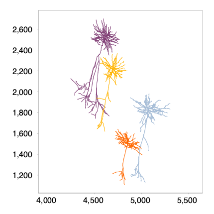
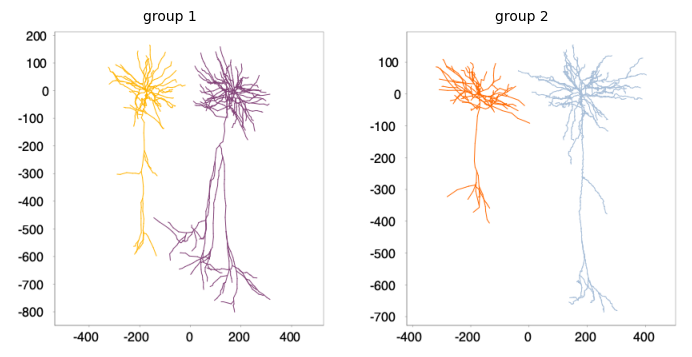
To display the groups, we can use the same strategy as before:

viewers = [] # visualization result: 1 viewer per group

for group in g_stats.getGroups():

    # Retrieve the trees in the group
    group_stats = g_stats.getGroupStats(group)
    group_trees = group_stats.getGroup() 

    # Define a viewer for the group
    viewer = Viewer2D()
    
    # Normalize absolute coordinates and rotate cells so their main axis is vertical
    group_trees_transformed = Tree.transform(group_trees, "zero-origin upright-geodesic", False)
    
    # Assign the group color and offset each tree by 350µm left/right
    # for better visualization
    n_trees = len(group_trees_transformed)
    for i, transformed_tree in enumerate(group_trees_transformed):
        # Calculate offset: negative for first half, positive for second half
        offset = (i - (n_trees - 1) / 2) * 350
        transformed_tree.translate(offset, 0, 0)
    
    # Add transformed trees to viewer and store result
    viewer.add(group_trees_transformed)
    viewer.setTitle(group)
    viewers.append(viewer)

pysnt.display(viewers, show_panel_titles=True)

{'type': matplotlib.figure.Figure,
 'data': <Figure size 700x350 with 2 Axes>,
 'metadata': {'source_type': 'Viewer2D_List',
  'viewer2d_count': 2,
  'displayed_count': 2,
  'panel_layout': 'auto',
  'title': None},
 'error': None}

Summary and Next Steps

That concludes this tutorial. Have a look at remaining tutorials for further examples.

Data Sources and References

Data used in this notebook is part of SNT’s demo datasets. In particular, Dendrites of cells AA001, AA002, AA0003, and AA0004 of the MouseLight database, under a Creative Commons Attribution 4.0 International License (CC BY 4.0).

See SNT citation for details on how to properly cite SNT.